Growth, Cycles & Hysteresis

Until recently the US was special

A few days ago, David Beckworth did an interview with Antonio Fatás “Antonio Fatás on Hysteresis and the Business Cycle”.

The interview was based on Fatás’ recent paper “Hysteresis and Business Cycles” where the abstract reads:

Traditionally, economic growth and business cycles have been treated independently. However, the dependence of GDP levels on its history of shocks, what economists refer to as “hysteresis,” argues for unifying the analysis of growth and cycles.

In this paper, we review the recent empirical and theoretical literature that motivate this paradigm shift. The renewed interest in hysteresis has been sparked by the persistence of the Global Financial Crisis, as GDP in advanced economies remains far below the pre-crisis trends.

The findings of the recent literature have far-reaching conceptual and policy implications. In recessions, monetary and fiscal policies need to be more active to avoid the permanent scars of a downturn. And in good times, running a high-pressure economy could have permanent positive effects.

I highlighted “sparked by the persistence of the Global Financial Crisis…” because “names” matter. By calling the Great Recession (GR) “Global Financial Crisis” (GFC) you march to the wrong conclusion! At least one very different from the conclusion you get if you rightly (I think) attribute the GR to a massive monetary policy error that was never fully righted!

In developing my story, I will make connections to bits of Fatás’ comments on the interview with Beckworth.

Fatás: When it comes to empirical work, there's an empirical fact that we all accept, I think almost all of us accept, which is fluctuations are persistent. So typically, when there's a shock, when there is a recession, if you look at the long-term effect of that recession, it is somewhere in there or over a long horizon. So we do not go back to a linear trend. So we don't go back to a pre-crisis linear trend.

Fatás: And I think this goes back to the unit root discussions that date back many, many years ago. And I think again, in most time series analysis of U.S. GDP, I think that's what we see. We see a very persistent fluctuation. Now, that matches the notion of hysteresis, that when you have a shock, the shock is not just cyclical, it becomes permanent. But of course it also matches the workhorse model in business cycles, which is the real business cycle model, because in that model shocks are permanent by definition because they affect technology.

Fatás: They affect the parameter in the production function. So then it becomes a little bit of a race. Here, you have two predictions about permanent effects of cyclical shocks. One is about the exogenous component is permanent. The other, the hysteresis story is the endogenous reaction of the economy makes a cyclical shock permanent.

Fatás: So a lot of the empirical literature has been about a fight between these two stories, because I think that persistence of fluctuations is obvious in the U.S. and it's even more obvious outside of the U.S. So again, it doesn't matter which country you look at. The debate is what causes that persistence? Is it supply shocks? Is it the exogenous persistent or is it the hysteresis endogenous reaction to a cyclical shock?

The theme here is the persistence of fluctuations, and that they are obvious in the US (and even more obvious in other countries).

The chart below covers 140 years of US real output (RGDP). The trend line (dotted line) was formed between 1880 and 1928, right before the Great Depression occurred.

If you were standing in 1928 and “believed” the trend to that point was permanent (the trend indicates that RGDP growth evolved at a 3.4% per year click), your forecast for the year 2000 say, would only overestimate actual 2000 RGDP by 125 billion dollars (a 0.95% error! Any doubt that your name would go to the Guinness Book as the best forecaster on earth?).

Of course, you would be laughed off the stage for missing the 2 year forecast by 18%! The important thing to note is that, contrary to what Fatás says, we did go back to a pre-crisis linear trend.

The next charts show RGDP & Trend with quarterly data since 1954. The red dotted line is still the 3.4% growth trend. The green dotted line is the RGDP 2.3% growth since the end of the GR. The RHS chart is just a zoom in of the LHS chart covering the post GR period.

Given that after the GR both the level and growth rate of RGDP remained well below the pre GR trend level and growth, it appears Hysteresis has finally caught up with the US economy. More on that later.

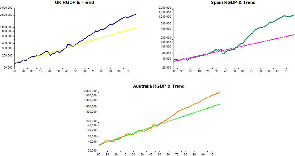
While “persistence of fluctuations were not obvious in the US prior to 2008”, they certainly were obvious in a host of other counties. The next chart shows how different from a “trend stationary” process like the US the RGDP of the UK, Australia and Spain behaved. (for these countries the trend is also formed between 1880 and 1928).

I am not getting into a technical discussion of these alternative processes, but want to note a couple of points. One is that in all these countries, RGDP “departed” from their earlier trend shortly after the end of WWII. The other is that their processes thereafter is quite different. Compare, for example Spain and Australia.

In Spain fluctuations appear much more persistent, and hysteresis may be present. Note, specifically, that since the GR, you don´t notice a clear break in Australia, but it is clear in Spain (and also in the UK). Remember that the same break is present in the US RGDP series after 2007.

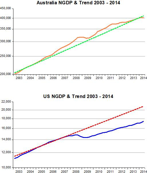
I believe you can relate that difference between Australia on the one hand and the US, Spain & UK on the other, to the behavior of monetary policy. And if monetary policy (the stance of which is gauged by Aggregate Nominal Demand (NGDP) growth) can “explain” the difference in outcomes, we should not fall prey to hysteresis arguments (at least for the US), but go back to the drawing board to develop better monetary policies.

The chart shows the very different behavior of monetary policy in Australia and the US (the same goes for UK and Euro Zone (to which Spain belongs)) around the Great Recession. It´s really more of a massive monetary blunder than a GFC. When the central bank allows nominal spending tank so abruptly, the economy will pay a high price.

The US economy had already payed an even much higher price in the Great Depression. The US recovery that brought RGDP back to the linear trend path it was on before is mostly due to the expansion of monetary policy that occurred after Roosevelt devalued the dollar and left the gold standard in March 1933.

This time around, monetary policy was “passive”, content to allow NGDP remain on the lower trend path it had dropped to. RGDP follows suit! In that sense, the persistence of the monetary shock gives rise to what Fatás calls hysteresis.

We can only wonder what the Fed will do following the Covid19 shock. It is still short of allowing RGDP climb to the “depressed path” it was on after the GR. With many very worried about inflation, I´m not very optimistic. And the new jargon of “high pressure economy” or “overheating” is not helpful.

Another bit of the Fatás interview I found interesting and that I find also nicely relates to monetary policy is this:

Fatás: I think to me, in the current debate, here is what I would like to combine hysteresis with an asymmetric view of the business cycle. Because if you combine the two, then you can make a very strong point. Again, I go back to the previous expansion. It took us 10 years to bring the unemployment rate down to 3.5 in the U.S. Now, that is really not what our economic models predict that you get a shock and it takes a 10-year expansion to go back to normal, to full employment. Why is that not that what our models predict?

Fatás: Because this was the longest expansion ever. If the longest expansion barely took us to full employment, what happened in all the previous ones? Did we ever get there? And this is fundamental question that we, as economists, have not answered yet at least not according to my taste. And this goes back to the plucking model. Do we go back to full employment ever? I'm writing a paper on this right now. We never seen the U.S. a period of low unemployment that persists for years. We've never seen it.

Fatás: Look at the picture of unemployment in the U.S., every time it goes low, it jumps back up. Again, that's not what our models predict. So again, that's the plucking model. There's no hysteresis there. Now, add hysteresis to that and you say, "Well, during those years where unemployment was too high, we were not at potential." If you believe there is hysteresis, we're damaging the long-term potential of the economy little by little. By how much? We don't know yet but certainly there must be some effects on the supplier of the economy. Now, what we're doing this time in the U.S. is let's go as fast as we can towards potential.

Fatás: Now, to me, that sounds like a good idea given that last time it took us 10 years and 10 years sounds suboptimal I think for all of us. And then, yes, let's see how far we can push that potential output. We all know it's very hard to measure potential output. We all know our measures of potential output tends to be incredibly cyclical. In recessions, we all become pessimistic and we immediately lower potential output. But if you have a very strong boom, and in the case of the U.S., I think that's the 1990s, you can keep raising potential output as you go along. So where that line is, I think we need to admit there's a lot of uncertainty.

The point I want to discuss is this; “Look at the picture of unemployment in the U.S., every time it goes low, it jumps back up. Again, that's not what our models predict.”

I think it´s exactly what “our models” predict, especially those that involve the Phillips Curve in one way or another (think New Keynesian Models, for example). Policy makers have a view of what the “natural rate” of unemployment is, so when unemployment gets close (or surpasses that level), monetary policy (i.e. NGDP growth) is constrained, so the unemployment rate goes up.

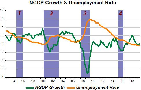
The next chart shows that keeping NGDP growth on a stable path leads to a continuous fall in the unemployment rate. The level along which spending growth evolves determines the overall “quality” (employment ratios, participation rates of all segments, among others) of the labor market.

Note, in particular, how sensitive unemployment is to fluctuations in NGDP. Small fluctuations (1,4) will only stop the fall in the unemployment rate. A large fall in NGDP growth will have a significant effect (2), while a massive drop will have “catastrophic” effects (3).

What the Fed is doing now is “groping in the dark”, not “ go as fast as we can towards potential”

As I argued here, the Fed (and other central banks) should make their choices explicit, and then “get to them as quickly as possible”!