
The "relative price - inflation" confusion
The "relative price - inflation" confusion
incites bad monetary policy moves

John Cochrane has written “Inflation confusion” a detailed critical comment on the WSJ piece “Why Inflation Is Biden’s Most Stubborn Political Problem”
In a nutshell, it is the most stubborn political problem because they think “jawboning” (fighting inflation by applying political pressure to companies not to raise prices) is the only solution, forgetting that this “policy” was amply and unsuccessfully applied during the great inflation.
The attention of analysts and pundits on individual prices has been overwhelming. Just to give two recent favorites as example: Health care costs and auto insurance.
It is well known that Cochrane has an “inflation is a fiscal phenomenon” bias (recently he published a textbook titled “The Fiscal Theory of the Price Level”).
His bias comes out clearly in this quote:
For all of the excess stimulus under Trump, the fact is that inflation broke out precisely in February 2021, and not a minute beforehand. If you want an event, the Feb 2021 “American Rescue” act, with a few trillions more stimulus though the pandemic was clearly over, made clear that this administration was not going back to standard fiscal policy.
Yes, inflation broke out precisely in February 2021 as the chart below attests.

This “timing” is more general, also affecting the Harmonized version of the CPI which excludes Owners Equivalent Rent (OER). (OER is also present, with a significantly lower weight in the PCE).
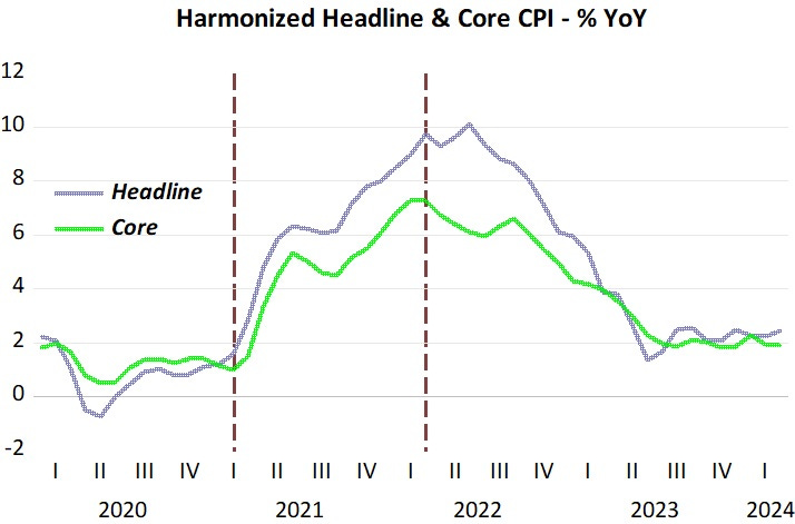
Note that the headline HCPI rises for longer, with this being due to the lingering effect of the oil price shock due to the Russian invasion of Ukraine.
If the American Rescue Act was responsible for inflation taking off (because “it became clear the Administration was not going back to standard fiscal policy”), what made inflation peak and began to fall in March 2022 if perceptions of fiscal policy have not changed?
In contrast to the “fiscal view”, the “monetary view” accounts for both the rise and the fall in inflation, with the timing being “precise” (i.e. no lags!).
From the equation of exchange MV=PY, where M is the money supply, V is velocity, P the price level and Y real output, in growth form, we can appeal to the “Thermostat Analogy”.
A good thermostat (M, closely controlled by the Fed) is one that manages to offset changes in the “outside temperature” (V) so as to keep the “inside temperature” (PY or NGDP) stable.In the charts below, we observe that inflation takes off at the precise moment that velocity takes off (money demand falls) and money supply growth is not reduced enough to offset the rise in velocity. The result is that NGDP growth spikes and inflation takes off.

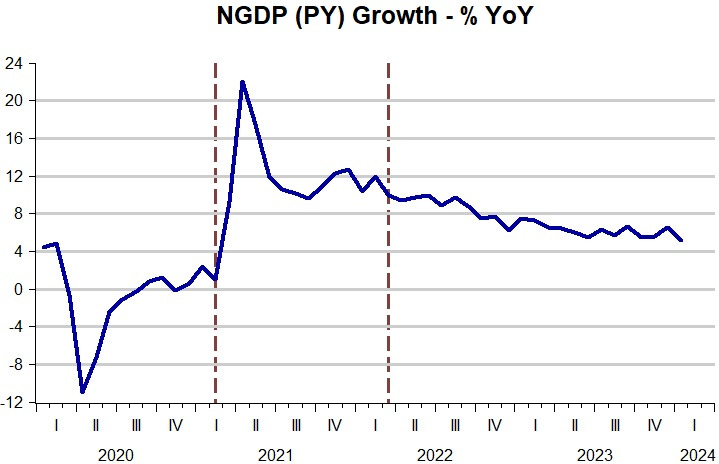
Also, inflation begins to fall at the precise moment that money supply growth begins to fall (even turning negative) while velocity growth remains relatively stable. NGDP growth slides down from close to12% to 5%.
The Fed has (even if unwittingly) approached nominal stability, with better gauges of inflation having remained close to 2% for several months. Going forward the Fed had better stop talking too much about the timing of interest rate reduction and concentrate on keeping NGDP growing in the 4.5% - 5% range. Meanwhile, the President´s advisers, especially the CEA, who should know better, stop the useless, likely harmful, “jawboning” tactics.
The G.6 release fell to President Bill Clinton’s “Paperwork Reduction Act of 1995”: From the Federal Register:
“The usefulness of the FR 2573 data in understanding the behavior of the monetary aggregates has diminished in recent years as the distinction between transaction accounts and savings accounts has become increasingly blurred (And that’s also what Chairman Alan Greenspan said about M1). But Vt would have stuck out like a sore thumb with the boom in real-estate.
Further, the emphasis on monetary aggregates as policy targets has decreased. In addition, respondent participation has declined over the last several years. For these reasons, the Federal Reserve proposes to discontinue the survey and the related statistical release.”
That was exactly why the G.6 Debit and Demand Deposit Turnover statistical release should not have been discontinued by Ed Fry (then the BOG’s longest running time series).
Vi is a “residual calculation - not a real physical observable and measurable statistic.” Income velocity may be a "fudge factor," but the transactions velocity of circulation is a tangible figure.
I.e., income velocity, Vi, is endogenously derived and therefore contrived (N-gDp divided by M) whereas Vt, the transactions’ velocity of circulation, is an “independent” exogenous force acting on prices.
Money demand is viewed as a function of its opportunity cost-the foregone interest income of holding lower-yielding money balances (a liquidity preference curve). As this cost of holding money falls, the demand for money rises (and velocity decreases).
As Dr. Philip George says: “The velocity of money is a function of interest rates”
As Dr. Philip George puts it: “Changes in velocity have nothing to do with the speed at which money moves from hand to hand but are entirely the result of movements between demand deposits and other kinds of deposits.”
The track of inflation has been textbook. There have been no surprises.