The nominal economy leads

and inflation is not a price phenomenon as Krugman has realized

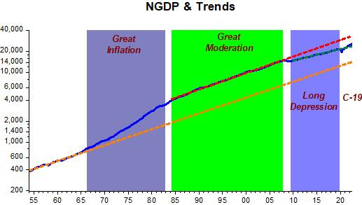
Below a description of the nominal economy (aggregate nominal spending or NGDP) with “identifying stamps” over the past 70 years.

Until the mid-1960s, NGDP was on a stable growth path. The Great Inflation comes about when aggregate nominal spending goes on a “spree”, rising at an increasing rate. In the mid-1980s NGDP resumes the stable growth path that characterized the pre GI period, with the growth rate observed along this path being the same as the pre GI growth rate (the red and orange trend lines are parallel). The nominal spending level is higher because the price level permanently rose during the Great Inflation (and to bring the price level down would be tantamount to “economic hara-kiri”!)

The “Long Depression” comes about when the aggregate nominal spending level drops and then rises at a lower growth rate. As will be “picture clear” later, C-19 threw sand in the “spending machine”, making it go “haywire”.

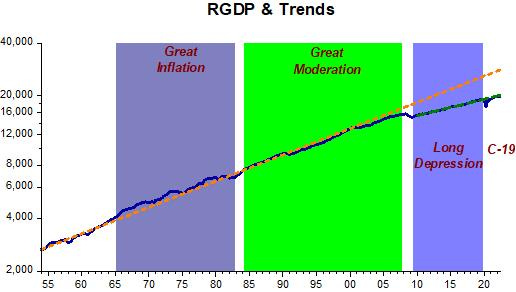
The nominal picture above has a real counterpart which describes the behavior of quantities (real output).

Prior to the mid-1960s, with aggregate nominal spending flowing along a stable path, RGDP remained close to its “potential” path defined by the trend line. There are a couple of “down wiggles” representing the recessions of 1957 and 1961, but real output recovers quickly to trend.

The Great Inflation changes the pattern. During that period, RGDP remains mostly above the trend path and recessions during that time (1970, 1973-75, 1980) are occasions when real output falls back to trend. During the last recession of that period (1981-82), RGDP falls below trend. After a quick recovery back to trend, real output remains very close to the trend path for more than two decades, receiving the moniker “Great Moderation”. ( Please don´t fail to note the nominal stability that characterizes this period, made clear in the NGDP level chart).

Note that after the recessions of 1990-91 and again after the recession of 2001, both “shallow & short” RGDP takes a long time getting back on trend after the first and doesn´t get a chance to fully recover after the second, being “jostled” into the “Long Depression”. As I´ll argue later, the Fed´s “print” is all over those happenings.

During the “Long Depression”, the Level of real output is permanently reduced, the same being said about its growth rate. No wonder talks of a “New Normal” or “Secular Stagnation” became “popular”.

As will also be “picture” clear later, C-19 threw sand, this time in the “producing machine”, making it go “haywire”.

The next two pictures are the growth rate counterpart of the first two charts.

Some comments on the growth charts:

There´s no summary statistics for NGDP growth during the Great Inflation because nominal spending growth is not stationary, showing a rising trend, so that mean and standard deviation are not defined.

The dotted circle in the first half of the 1960s “identifies” what I´ll call the “Camelot Dream”. During those few years, nominal and real growth are consistently high and relatively stable.

In his 1972 Eliot Janeway Lectures Nobel Prize James Tobin, an active participant, writes that “to return to Camelot (as President Kennedy Council of Economic Advisers was known) is to revisit an era when growth was a good word, indeed the good word…”.

According to Arthur Okun (1970), an active participant, first as staff member and later Chairman of the Council of Economic Advisers (CEA), in the economic decisions throughout  the decade:

“The strategy of economic policy was reformulated in the sixties. The revised strategy emphasized, as standard for judging economic performance, whether the economy was living up to its potential rather than merely whether it was advancing…the focus on the gap between potential and actual output provided a new scale for the evaluation of economic performance, replacing the dichotomized business cycle standard which viewed expansion as satisfactory and recession as unsatisfactory. This new scale of evaluation, in turn, led to greater activism in economic policy: As long as the economy was not realizing its potential, improvement was needed and government had a responsibility to promote it. Finally, the promotion of expansion along the path of potential was viewed as the best defense against recession. Two recessions emerged in the 1957-60 period because expansions had not had enough vigor to be self-sustaining. The slow advance failed to make full use of existing capital; hence, incentives to invest deteriorated and the economy turned down. In light of the conclusion that anemic recoveries are likely to die young, the emphasis was shifted from curative to preventive measures. The objective was to promote brisk advance in order to make prosperity durable and self-sustaining…The adoption of these principles led to a more active stabilization policy. The activist strategy was the key that unlocked the door to sustained expansion in the 1960s”.

But Okun also recognizes that:

“The record of economic performance shows serious blemishes, particularly the inflation since 1966. To some degree, these reflect errors of analysis and prediction by economists; to a larger degree, however, they reflect errors of omission in failing to implement the activist strategy”.

(Funny how often policymakers and commenters fall prey to the “it wasn´t enough” argument, in this case not “activist enough” or, more recently, “the 2009 fiscal stimulus wasn´t big enough”.)

In a 1936 review of “Keynes on Unemployment”, Jacob Viner conjectured that:

“Keynes’ reasoning points obviously to the superiority of inflationary remedies for unemployment over money-wage reductions. In a world organized in accordance with Keynes’ specifications there would be a constant race between the printing press and the business agents of the trade unions, with the problem of unemployment largely solved if the printing press could maintain a constant lead and if only volume of employment, irrespective of quality, is considered important”.

This seems consistent with what transpired in the 1960s, when we take into account the fact that to Arthur Okun:

“The stimulus to the economy also reflected a unique partnership between fiscal and monetary policy. Basically, monetary policy was accommodative while fiscal policy was the active partner. The Federal Reserve allowed the demands for liquidity and credit generated by a rapidly expanding economy to be met at stable interest rates”.

By the mid-1960s, the policymakers began to have doubts. According to Arthur Okun:

“In 1965 the nation was entering essentially uncharted territory. The economists in government were ready to meet the welcome problems of prosperity. But they recognized that they could not provide a good encore to their success in achieving high-level employment”.

And as Gardner Ackley, then CEA Chairman put in a talk on “The Contribution of Economists to Policy Formation” delivered in December 1965:

“…The plain fact is that economists simply don´t know as much as we would like to know about the terms of trade between price increases and employment gains (i.e, the shape and stability of the Phillips Curve). We would all like the economy to tread the narrow path of balanced, parallel growth of demand and capacity utilization as is consistent with reasonable price stability, and without creating imbalances that could make continuing advance unsustainable. But the macroeconomics of a high employment economy is insufficiently known to allow us to map that path with a high degree of reliability…It is easy to prescribe expansionary policies in a period of slack. Managing high-level prosperity is a vastly more difficult business and requires vastly superior knowledge. The prestige that our profession has built up in the Government and around the country in recent years could suffer if economists give incorrect policy advice based on inadequate knowledge. We need to improve that knowledge”.

The result of a continuously expansionary monetary policy, reflected in the rising growth of nominal spending, led us to the “Great Inflation”, which in the 1970s was made worse by the economy being buffeted by a series of supply shocks, in addition to wage & price controls and exchange rate fluctuations due to the end of the fixed exchange rate regime in 1971-73.

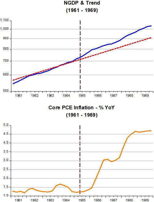
The chart below zooms in on the 1961-69 period and shows the effect on inflation of “Camelot economic policies”.

Moving on, the Great Moderation was characterized by robust real growth with a volatility that was half of that experienced previously. The “Long Depression” (or “Depressed Moderation”) was characterized by significantly lower nominal and real growth with volatility little changed.

As I mentioned above, after the recessions of 1990-91 and again after the recession of 2001, both “shallow & short” RGDP takes a long time getting back on trend after the first and doesn´t get a chance to fully recover after the second, being “jostled” into the “Long Depression”.

Recently, Joe Gagnon wrote 25 years of excess unemployment in advanced economies: Lessons for monetary policy

For about 25 years before the COVID-19 pandemic, inflation was very low and stable in most advanced economies. A little noticed dark side of this impressive achievement is that unemployment rates were almost always higher than needed to keep inflation low. This widespread and persistent policy error arose because of a major flaw in standard macroeconomic models—the use of a linear Phillips curve.

He suggests that the inflation target should be higher! In my view the problem arises from using the Phillips Curve framework for controlling inflation, which is perceived to be stoked by a “too low” unemployment rate.

So the reader has an idea about the importance of the Phillips Curve concept in the Fed´s policy making apparatus, this is from one of the first speeches made by Laurence Meyer in April 1997, shortly after being made Fed Governor (the FOMC had increased the FF rate by 25 basis points in March, after rates having been left unchanged for a little over one year):

Utilization rates in the labor market play a special role in the inflation process. That is, inflation is often initially transmitted from labor market excess demand to wage change and then to price change.

This principle may be especially important today because, in my view, there is an important disparity between the balance between supply and demand in the labor and product markets, with at least a hint of excess demand in labor markets, but very little to suggest such imbalance in product markets.

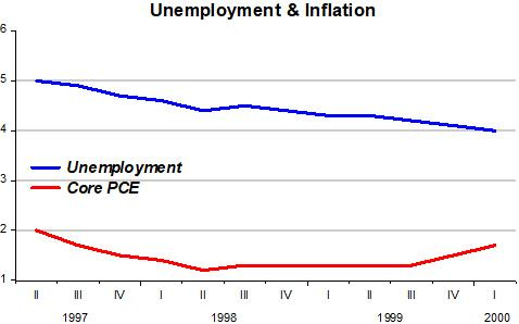
To prove Meyer wrong, the chart shows what happened to unemployment and inflation in the three years following his speech.

At least one FOMC member, William Poole, President of the St Louis Fed learned something from that period. In the June 2000 FOMC Meeting he made what is to me, one of the most insightful comments in FOMC Meetings history:

The traditional NAIRU formulation views the wage/price process as running off a gap–a gap measured somehow as the GDP gap or the labor market gap. And the direction of causation goes pretty much from something that happens to change the gap that feeds through to alter the course of wage and price changes.

I think there is an alternative model that views this process from an angle that is 180 degrees around. It says that in an earlier conception, monetary policy pins down the price level or the rate of inflation and, therefore, expectations of the rate of inflation. 

Then the labor market settles, as it must, at some equilibrium rate of unemployment. Where the labor market settles is what Milton Friedman called the natural rate of unemployment.

But the causation goes fundamentally from monetary policy to price determination and then back to the labor market rather than from the labor market forward into the price determination. I certainly view the causation in that second sense.

Now, the labor market has been clearing at a level that all of us have found surprising. But I don’t think that necessarily has any particular implication for the rate of inflation, provided we make sure that we are willing to act when necessary. (pg 61).

The panel below provides a clear illustration of Gagnon´s argument that “unemployment rates were almost always higher than needed to keep inflation low”.

Looking at the left-hand side of the panel, the color-coded arrows indicate that as soon as unemployment fell to levels deemed close to what was thought to be the “natural” level, monetary policy tightened, as indicated by the fall in NGDP growth.

At those times unemployment rose and the right-hand side charts indicate that a recession ensued but nothing untoward was happening to inflation!

This explains the fact I noted early on in this post “that after the recessions of 1990-91 and again after the recession of 2001, both “shallow & short” RGDP takes a long time getting back on trend after the first and doesn´t get a chance to fully recover after the second”.

The “Long Depression” (or “Depressed Moderation”) was the result of a gargantuan monetary policy error. First, the Fed under Bernanke allowed NGDP growth to become significantly negative and then, never allowed NGDP to get back to the “Great Moderation” trend, keeping it at a lower level path and growing at a reduced rate.

No wonder unemployment took such a long time to fall back! Contrast that with the very rapid drop in unemployment after the C-19 shock, which was the result of a very different monetary policy, one which allowed NGDP to quickly get back to the post “Great Recession” trend!

Going into the C-19 period, note that this shock is very different from what was experienced previously. The sudden and very wide swings in nominal spending and real output are unprecedented.

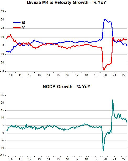
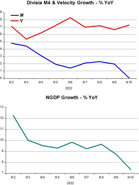
To make things visually clear, the next charts show that during the post Great Recession period, from 2010 to 2019, monetary policy was adequate to keep NGDP growth stable close to 4% yoy. That was the outcome of money supply appropriately offsetting changes in velocity.

Suddenly, a velocity shock (from C-19) hit. Money supply reacted quite quickly, so the recession was the shortest on record (2 months). That was the nominal effect of C-19. There were also real effects, from lockdowns, supply chain dismantling, demand composition disturbances, among others. (Much later another real shock, from the Russia invasion ensued).

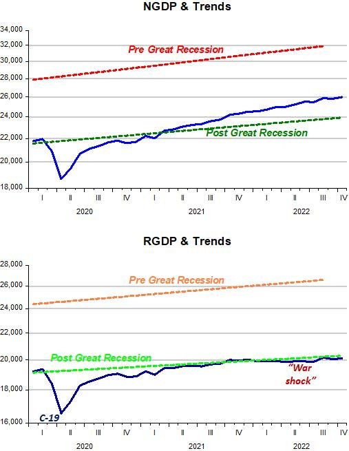
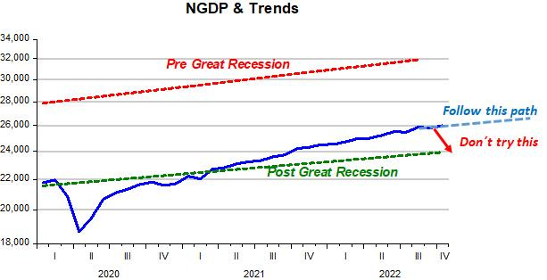
The level charts illustrate in more detail. Note the quick recovery from the C-19 shocks. Note also the impact of the Russian invasion shock (when many thought the US had entered a recession).

The “talk of the town”, however, has been inflation. In his most recent speech - Inflation and the Labor Market - Powell indicates he never read William Poole´s comments in the 2000 Fed Transcripts noted above because he continues to favor Laurence Meyer´s argument that:

Utilization rates in the labor market play a special role in the inflation process. That is, inflation is often initially transmitted from labor market excess demand to wage change and then to price change.

Saying:

In the labor market, demand for workers far exceeds the supply of available workers, and nominal wages have been growing at a pace well above what would be consistent with 2 percent inflation over time. Thus, another condition we are looking for is the restoration of balance between supply and demand in the labor market.

In contrast to Powell´s “mainstream” Phillips Curve view, Brad DeLong has a “juicy” but very sensible view:

The inflation we have had over the past two years has been, largely, a good thing—or, rather, a necessary consequence of a very good thing. Not to have had an inflation surge as we reopened the economy after the plague—that would have been to run unacceptably high risks of a repeat of the disastrously slow recovery of the Obama years. Moreover, we needed wage inflation in the goods-producing, logistics, and information sectors in order to pull workers returning to work into the sectors that needed to expand to get the economy to full employment given the altered post-plague shape of demand. And we needed inflation at the bottleneck breaks in supply chains to incentivize their repair.

After discussing in detail price/inflation components, Paul Krugman realizes that this sort of analysis is not helpful in identifying “underlying inflation”:

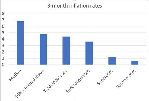
At this point, however, various measures of core inflation are all over the map. Here’s a picture of inflation rates over the past three months (calculated as annual rates of change) for six measures I’ve been following…

OK, depending on which measure you choose, underlying inflation is anywhere from almost 7 percent — way above the Fed’s target — to less than 1 percent, well below the target. That’s not helpful!

I don’t think this is mainly a data problem. What we have, instead, is a conceptual problem: What do we mean by “underlying” inflation, anyway?

One possible answer is that it means inflation driven by generally excessive spending rather than issues specific to particular sectors of the economy.

Concluding:

So where are we on the inflation fight? Until recently it was clear that overall spending was rising too fast to be consistent with low inflation, and my superdupercore measure suggests that this may still be true. I certainly understand why the Fed isn’t ready to declare victory yet.

But given the absence of evidence that inflation is getting entrenched, victory may be a lot closer than many people imagine.

And I believe it is! Why? So here´s a story:

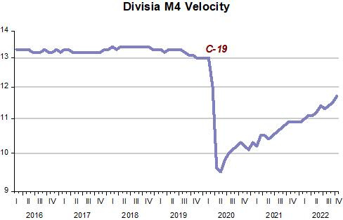
I´ve said that one aspect of the C-19 shock was a massive velocity shock. This is clearly shown in the chart.

Since the recovery began, velocity has been climbing back to its stable level. A changing velocity certainly makes monetary policy harder, since Nominal Stability requires that the Fed “calibrates” the money supply to offset changes in velocity.

Since early this year, the Fed appears to have “gotten the hang of it”, with monetary policy (don´t confuse with interest policy) offsetting the change in velocity so as to bring spending (NGDP) growth down.

More recently, traditional monetarists have stopped “worrying” about inflation and are predicting a coming deep recession from the absence of any money growth, failing to account for the rising velocity! (Just as in mid-2020 they were predicting “monster” inflation from the “massive” increase in money growth, failing to account for the also “massive” drop in velocity).

One scenario going forward is if velocity continues to rise back to its “normal” level at the average rate of 6.5% that has been observed since mid-2021, money growth will have to turn negative to bring spending growth closer to the 5% rate that has been the decades-long “norm” consistent with a close to 2% inflation rate.

If that happens, a “soft-landing” will be a distinct possibility and a recession will be avoided.

The Fed should not “radicalize” and try to bring NGDP back to the post Great Recession trend path. That path was “artificial” anyway, being the outcome of the 2008 monetary policy mistakes. The best outcome is the “follow this path” alternative. As DeLong has suggested, the inflation we´ve had was good!