
The Great Recession from an Aggregate Demand Perspective
The Great Recession from an Aggregate Demand Perspective
Part 2

The previous arguments may be indicating that an IT regime may not be ideal. In the second half of the 1980´s several researchers, notably Bennett McCallum, with the purpose of devising “rules” for MP, discussed the idea that MP should be geared to maintaining stability in aggregate nominal expenditures (aggregate demand (AD)). This “search for rules” ended up being won by the proponents of the IT regime, with the interest rate (the FF rate in the US case) being the “instrument” of policy.
One of the effects of the ongoing crisis, characterized by an abrupt and steep fall in AD as will be seen below, was to bring back the discussion of what should be the target of MP. To the proponents of the view that the Central Bank should have as its objective the stability of AD, this is the “key” to macroeconomic stability – national or global.
For this group, shocks to AD are the true source of macroeconomic volatility while inflation is just a symptom of those shocks. Just like in medicine, symptoms may be related to different causes, so that prescribing the correct treatment is not trivial. In this sense inflation (a symptom) may be difficult to interpret: is inflation high (low) due to a positive (negative) shock to AD or to a negative (positive) supply (or real) shock? In situations of this kind, the prescribed “medicine” may not be the right one.
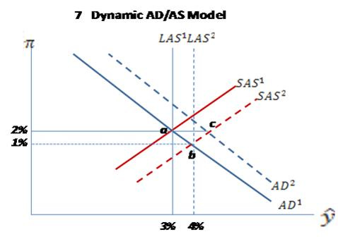
Figure 7 provides an illustration. The figure depicts the essence of a basic Dynamic Aggregate Demand/Aggregate Supply (AD/AS) model. The vertical axis denotes inflation while RGDP growth is depicted on the horizontal axis. The AD growth curve AD1 represents nominal expenditures growing at the rate of 5%. Along the AD1 curve the product of inflation and RGDP growth is 5%. The long run AS line LAS1 represents the growth of potential RGDP, which has been about 3% for the US over the last 50 years. The long run AS is vertical to reflect the fact that in the long run AS is determined by real factors. In the short run, however, the AS curve SAS1 is positively sloped due to temporary rigidity of prices and wages.
The dynamics of the level of RGDP and prices is illustrated in figure 8.
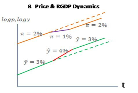
In the graphical model (fig. 7) the initial point is at a to which is associated an RGDP growth of 3% and an inflation rate of 2%. Let us suppose that the economy experiences a real, or productivity shock that permanently raises the level of potential RGDP (fig. 8). In this case the economy goes from point a to point b where RGDP growth increases to 4% and inflation falls to 1% with AD growth remaining at 5%.
To associate the model to real world events, some may recall that in the second half of the 1990´s there was a heated discussion about if the Fed was “behind the curve”. Several analysts, among them Paul Krugman, accused the Fed of being complacent with inflation by not raising the FF rate when RGDP growth was “clearly” above “potential’.
Greenspan would reply that the US economy was going through a period of higher productivity growth (a positive supply shock), that had temporarily increased the sustainable rate of output growth, something that did not call for an increase in the FF rate.
Note that in time the economy returns to point a with growth falling back to 3% and inflation moving back to 2%. The level of RGDP is permanently higher and the price level will be permanently lower.
This will be the outcome if the Fed keeps the growth of AD at 5%. However, if it strives to keep inflation at 2% after it falls to 1% as a result of the positive supply shock, increasing AD growth to AD2 the economy will move from point b to point c. Since at point c the economy will be growing above its potential, inflation pressures will appear so that AD will have to be constrained (FF will increase) in order to keep inflation on target. In this case RGDP and employment volatility will certainly be higher than if the Fed had operated to keep AD growth stable.
Panel 1 below depicts the theory described in the simple model (figures 7 & 8) above. While growth in the US economy was higher than what was considered “normal” by analysts, being the result of a higher rate of productivity growth, a fact that few other than Greenspan noted, the FF rate was stable and AD growth remained close to its average of a little more than 5%. After 1997, however, when inflation fell below the “target”, the Fed reduced the FF rate. AD went on to grow more than 7%.
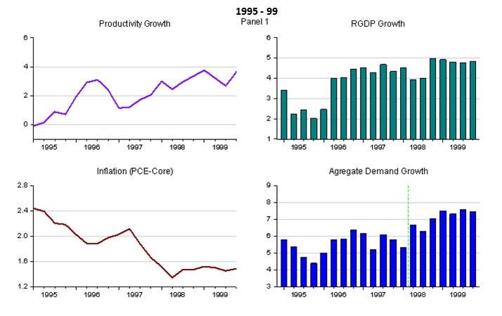
At this point RGDP growth climbs to close to 5% while inflation remains below “target”. Note that the trend growth of productivity is maintained over the period, indicating that the fall in inflation was the predictable outcome of positive supply shocks.
From reacting to an inflation below “target” reducing the FF rate in 1998, the Fed than reacts to an RGDP growth considered “exuberant”. So, when the unemployment rate falls below 4% in 1999 the Fed caved in to “popular demand” and raised the FF rate.
Panel 2 describes what happened next.
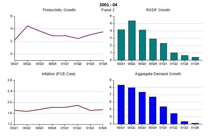
The main point to note is the strong reversal of AD growth. Inflation remains below the target and productivity growth remains strong. RGDP growth falls towards zero with 2001 being officially defined as a recession year.
AD instability after 1998 is associated with Fed actions. First the Fed reacted to a below target rate of inflation and then, in the opposite direction, reacted to an exuberant RGDP growth rate. This is indicative that an IT regime has an important flaw that manifests itself when the economy experiences supply shocks (also called real or productivity shocks).
Furthermore, we cannot discard the fact that a Fed induced AD instability also has consequences for asset prices. This is shown in figures 9 & 10 where we observe the strong positive correlation between AD growth and the NASDAQ and S&P stock indices.
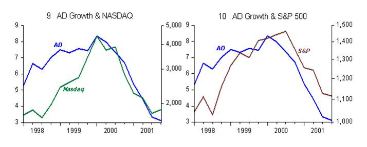
Note that the NASDAQ more than doubled between mid 1998 and early 2000 while the S&P rose by a little over 30%. This difference in the behavior of the two market indices is related to the fact that the NASDAQ, composed of technology stocks, was also influenced by the “productivity stories” of the time. Thus, what became known as a “bubble” was to a significant degree a reflection of AD instability.
So, if MP were to focus on stabilizing AD growth (level targeting), in addition to preserving macroeconomic stability it would also contribute to avoiding the appearance of “bubbles” in asset prices!
As was observed in figures 4 and 5, following the 2001 recession inflation remained low and unemployment high and rising with both reflecting the robust growth in productivity shown in Panel 2. Panel 3 describes how things unfolded in the 2002-05 period.
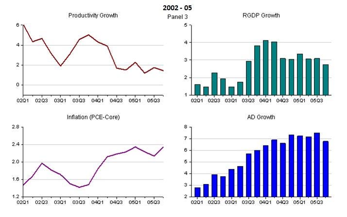
Expansion in AD only stabilizes (at the high rate of 7%) when inflation is brought back to “target”, the rate of unemployment is consistently falling and RGDP growth resumes its long run rate of about 3%.
As observed in figure 7 which illustrates the simple Dynamic AD/AS model, if MP is successful in keeping AD growth stable, the system adjusts while volatility remains low. If the Fed manipulates AD, influenced in turn by an inflation below target and then influenced by RGDP growth above potential, the system also adjusts – in the sense that inflation returns to target and growth to potential – but the shocks to AD resulting from these manipulations impart an undesired high level of volatility to the system, also affecting asset prices with spillovers (through wealth effects) to the real economy.
Given its size, events in the US economy have significant impact on the global economy. Figure 11 shows the behavior of AD (nominal expenditure growth) in the US over the last 50 years. It is relatively straightforward to associate this behavior to the periods that became known as “The Great Inflation” and “The Great Moderation”.
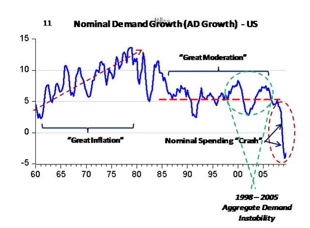
Figure 12 shows the similarity of the AD behavior in a group of 24 countries in the OECD. In the 1960´s and 1970´s the focal variable was the unemployment rate. During the Kennedy-Johnson administrations AD shocks, from MP and Fiscal Policy (FP), parted a positive bias to AD growth.
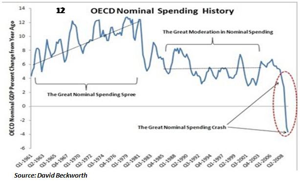
In the 1970´s, characterized by negative supply shocks (notably oil prices), increases in AD to compensate for the negative effects of the shocks on unemployment and RGDP growth resulted in high and rising inflation.
Panel 4 illustrates the “final sprint” to the crisis. As indicated in figure 3, in mid 2006 house prices began to fall. From this moment the delinquency rate began to grow affecting the health of important financial institutions. A few (New Century Financial, for example) went broke already at the beginning of 2007.
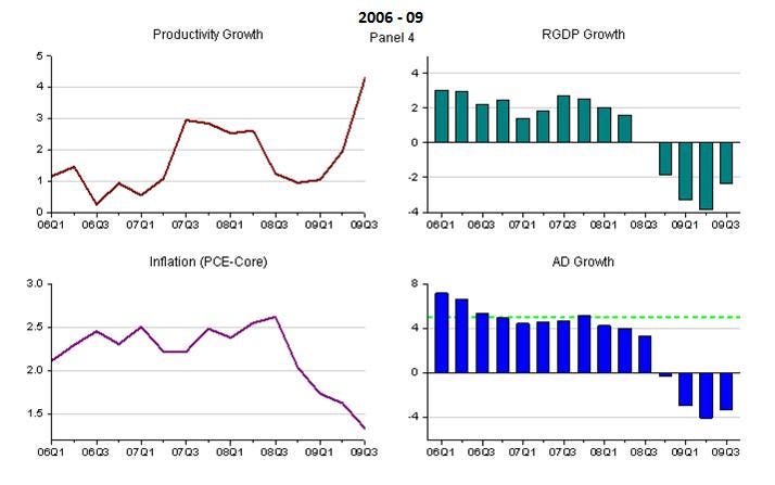
Notable, however, is the fact that between 2006 and mid 2008 AD growth was kept relatively stable and close to the trend path. Therefore, in spite of the crisis, the adjustments in the economy were able to proceed in an “orderly fashion”.
Observe in figures 13 and 14 that between 2006.II and 2008.II employment change was mostly positive and the unemployment rate remained stable. Something very different happens after 2008.II when AD “dives”, becoming negative for the first time since WWII. The change in employment is strongly negative and the unemployment rate shoots up.

Figures 15 and 16 help explain why it so happens that between mid 2006 and mid 2008 employment didn´t “dive” and the unemployment rate didn´t “soar”. With nominal spending growth (AD) relatively stable, resources flowing out of the residential construction sector were, among other, relocated to the export and non residential construction sectors.
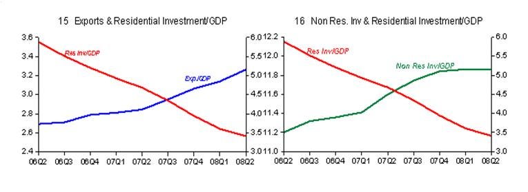
Only when AD “melts” is that a significant cyclical problem manifests itself. From this moment on the drop in economic activity is generalized and no “compensations” are possible.
It is interesting to note how many analysts see things in a completely different light. In a recent column in the Washington Post, for example, Alan Blinder who was a governor and vice chairman of the Fed (1994-96) and like Bernanke is a Princeton University professor writes that while between mid 2007 and mid 2008 Fed actions fell short, following the Lehman blow-up “the Fed deserves extremely high marks for its work since then. It has hit the bull’s-eye regularly under very trying circumstances”.
When it is said that the Fed regularly got it right at the same time that AD “melts down” something must be very wrong with people’s perceptions.
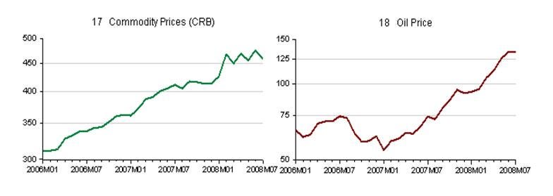
What is lacking is an explanation for the steep drop in AD. Once again the fact can be connected to the IT regime. Since early 2006 commodity prices were rising. In early 2007 oil prices joined in the fray, with price more than doubling in the next twelve months. Figures 17 and 18 illustrate.
Panel 4 showed that core inflation remained stable (even if slightly above target). The Fed feared that commodity and oil price increases would “infiltrate” the price system and push core inflation upwards.
The crisis gained the headlines in early August 2007 when three funds in Bank Paribas were closed for redemption. In the September FOMC meeting, in a gesture of “appeasement”, the Fed began a process of FF reduction. Nevertheless in every meeting after that the Fed always showed that it was very concerned with the risk of a rise in inflation. In the April 2008 meeting the FF rate was set at 2% and remained at that level until early October, when the “panic” set in.
In the August 2008 FOMC meeting, when commodity and oil prices had already turned down the Fed showed a very hawkish stance. One of the participants voted for an immediate increase in the FF rate and the release after the meeting indicated that the next move in the rate would likely be up! In the September 16 meeting, 24 hours after the collapse of Lehman and a few hours after receiving the news that industrial production had dropped by 1% in August, the Fed maintained the FF rate at 2% and reaffirmed its concern with inflation.
The Fed´s inflation fighting credibility – and the manifestations in the sequence of releases after meetings – indicated that the growth of nominal spending (AD) would be reduced in the future. Just like inflation expectations are an important determinant of present inflation, the same happens with AD growth.
The negative supply shock (from oil and commodity prices) and an IT regime meant that if the Fed strives to keep inflation at the “target” level it will contract AD growth. Given the Fed´s credibility, nobody doubted that that would happen. No wonder it did…
The financial crisis was certainly made worse by the expectation of a contraction in AD, and contributed to increase the economy´s “melt-down” rate.
I wonder in what kind of world we would be living today if 20 years ago the group that argued for the stabilization of AD growth (level targeting) as the rule to be followed by MP had won the debate over those that proposed IT with the interest rate as the policy “instrument”. Quite likely we would be experiencing much less “fiscal stimulus” with all its attendant risks.
As an end-note, Bernanke knows very well how to conduct MP at the ZLB. In a paper presented in 1999 (check Japanese Monetary Policy – A case of self-induced paralysis in the “Suggested Reading” list) he gave very useful advice to Japan (including “price level targeting”, a variant of AD targeting). One wonders why he did (and does) not take his own advice.