"Monetary Policy for Dummies"

30 years of visual "hard evidence"

The first thing to have in mind is that monetary policy should be concerned, exclusively, with the nominal economy. It should not be concerned, directly, with real variables such as employment/unemployment or real output. By taking good care of the nominal economy, it would be doing the best it can to keep the real economy in the best possible light!

What does “taking good care of the nominal economy” means? The logical answer is “monetary policy must strive to attain nominal stability”. That is more specific than just attain “price stability” (inflation on target) or “keep aggregate nominal spending - or NGDP - growing at a stable rate”. As we´ll see, the spending Level along wich aggregate nominal spending evolves is of crucial importance.

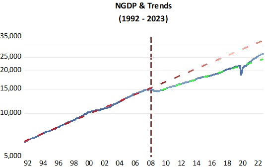
The first picture shows that over most of the last three decades, aggregate nominal spending (NGDP) evolved stably along two different level paths. The diving line between the two paths is the Great Recession. Further down the road, C-19 happened.

The contrast between the aftermath of those two “events” serves as a neat illustration of the power of monetary policy, when monetary policy is understood as the means to achieve and retain Nominal Stability.

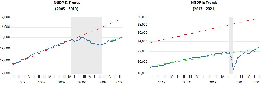
The next charts show what happened up to one year following the end of 1) the Great Recession, and 2) the end of the C-19 induced recession. The shaded areas define the period the economy was in recession according to the NBER, the official arbiter.

In the LHS chart, one year after the GR ended, the economy had begun “travelling” along a new, lower path. In other words, there was never a “recovery”! In the RHS chart, one year after the C-19 induced recession, deeper and more acute than the GR, aggregate nominal spending was back to the trend path that prevailed before the recession or, a full recovery in the short space of 12 months!

Why the huge difference? After the Great Recession, dubbed the “Great Financial Crisis (GFC)”, it became “fashionable” to argue that recoveries from financial crises are longer and protracted. See, for example, Why Was the Last Recovery Slower Than Usual? Actually, It Wasn’t

A new study of financial crises going back to 1870, coauthored by Arvind Krishnamurthy at Stanford Graduate School of Business, finds that the recession of 2007–09 played out pretty much as expected.

Regardless of whether government policy was helpful or not, the study finds, recessions triggered by financial crises have almost never been followed by snappy rebounds.

This other study, The Financial Crisis and Recovery: Why so Slow?, however, concludes the opposite:

Conclusion
The U.S. economy has only very slowly recovered from the recession of 2007 to 2009. U.S. history provides no support for an explanation based on the financial crisis itself, although data on financial crises in some other countries appear to do so.

The recent slow recovery is most similar to the Great Depression. Low aggregate demand for reasons unrelated to the financial crisis may be an explanation for both episodes, but uncertainty and government policies are an alternative supported by recent research on the Great Depression.

My own views are much closer to the second quote above. As I´ll argue later in this post, I go further and show that both the initial drop in spending and the subsequent path that spending followed is 100% the result of the monetary policy adopted.

The next charts show what happened to NGDP, or aggregate nominal spending, after the first anniversary of the GR and the C-19 recession, respectively.

In the first case, monetary policy led the economy to follow a lower trend path, with very stable spending growth (also at a lower rate than the one that prevailed before the GR (4% vs 5.5%, on average)).

In the second case, after bring spending back on trend in the first year following the C-19 recession, monetary policy allowed spending to rise above the trend.

In the first case, while monetary policy, which closely controls aggregate nominal spending, or NGDP, “established” a new, lower path along which the economy evolved stably, in the second case, monetary policy allowed spending to climb above the stable path it had reached.

In other words, while in the first case monetary policy attained nominal stability, even if, compared to the stability experienced during the Great Moderation, it could be called “Depressed Moderation”, in the second case monetary policy generated nominal instablity. Regaining nominal stability should now be the focal point of the Fed´s attention (more on that later).

Intermezzo

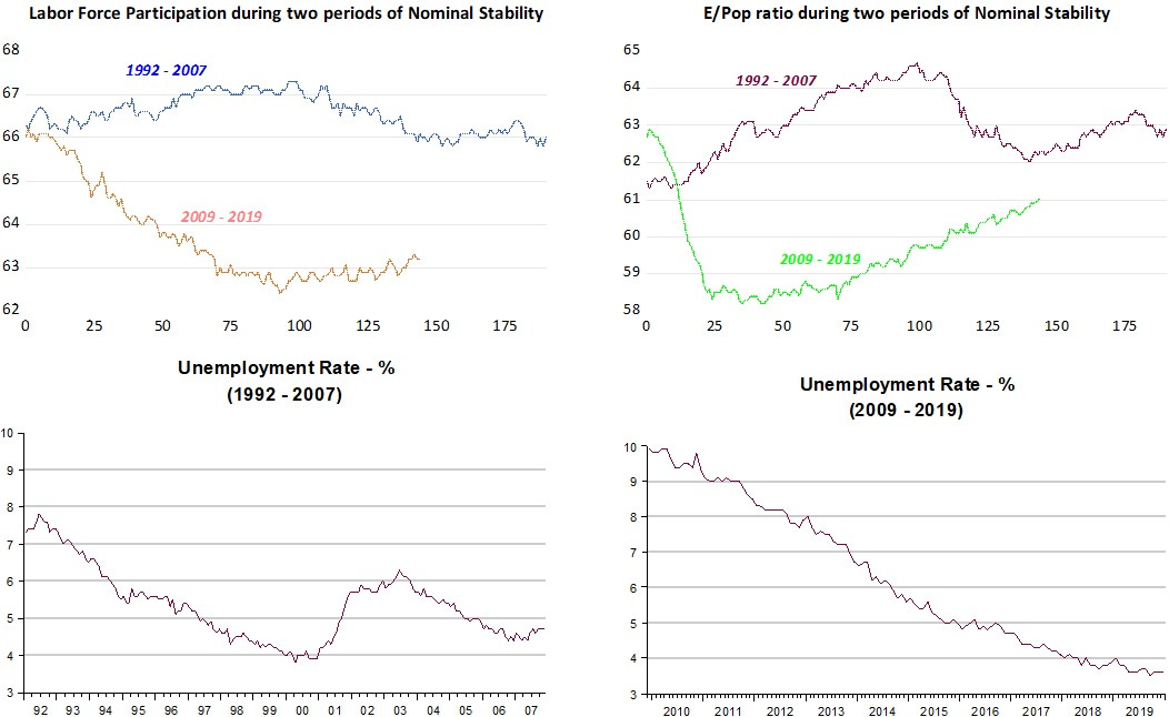
A break on the flow just to show how a “level break” on the trend path can have dire effects on the real economy, indicating the relevance of the Level of spending for monetary policy striving for nominal stability.

The charts show the two fundamental determinants of the unemployment rate; labor force participation and the employment population ratio. A “falling and/or low rate of unemployment” can be associated with a either a robust or weak economy, despite the fact that nominal stability is being actively and successfully pursued in both cases.

Monetary Policy

So far, I only have given a description of good and bad outcomes associated with monetary policy, but I haven´t defined what I mean by monetary policy. In my view, monetary policy is not to be confused with the Fed´s interest rate policy, where monetary policy is said to be “tightening” when the Fed is raising the Fed Funds rate, and is said to be “loosening” when the Fed is bringing the Fed Funds rate down.

Monetary policy, as the name suggests, is about money. Those who think so, however, are usually almost exclusively concerned with money supply, thinking monetary policy is “expansionary” when money supply growth is rising and that monetary policy is “tightening” when money supply growth is falling. In addition, to those who think monetary policy is about money, monetary policy is deemed “contractionary” when money supply growth is negative, meaning the stock of money is falling.

The “guiding light” to the monetary approach to monetary policy, is the equation of exchange: MV=PY or, in growth form m+v=p+y. This is an identity (just like the identity Y=C+I+G+(X-M) in the national accounts). We must, therefore, give it some structure (just like in the Y equation we give it some structure by, for example, assuming C and Y depend on income and interest rates and that government expenditures, G, is exogenous, to theorize about national income determination).

Quantity theorists give some structure to the equation of exchange by assuming that V (the inverse of money demand) is stable, so that v=0. In that case, we can rearrange the equation to get: m-y=p or, in words, “inflation is the result of too much money chasing to few goods”.

Further, since real output, Y (or y) in the long run is determined exclusively by real forces, in the long run inflation will be the only result of an increase in money growth.

As the quantity theory is structered, V is considered a residual in the equation, as it is the part that is left over after accounting for the other variables.

But, Milton Friedman himself said more than 50 years ago, “velocity can be anything people want”! So it´s nothing like it is “simply a residual”. (See, for example, Michael Bordo and Lars Jonung “Demand for Money - An analysis of the long-run behavior of the velocity of circulation).

In his 1971 JPE article “A monetary theory of nominal income”, Friedman asks:

What, on this view will cause the rate of change in nominal income to depart from its permanent level [or trend level path]?

Anything that produces a discrepancy between the nominal quantity of money demanded and the quantity supplied, or between the two rates of change of money demanded and money supplied.

In 2003, Friedman popularized that view with his “The Fed´s Thermostat” to explain the “Great Moderation”:

In essence, the newfound stability was the result of the Fed (and many other Central Banks) stabilizing nominal expenditures. In that case, from the equation of exchange, according to which MV=PY, the Fed managed to offset changes in V with changes in M, keeping nominal expenditures, PY, reasonably stable. Note that PY or its growth rate (p+y), contemplates both inflation and real output growth, so that stabilizing nominal expenditures means stabilizing both inflation and output.

Obs: Nick Rowe has a neat post on the Thermostat Analogy.

What I mean by monetary policy becomes clear. It means that the Fed is affecting the money supply so as to offset changes in velocity in order to keep aggregate nominal spending (NGDP) on a stable level growth path.

Imagine the economy is a house, the Fed the “thermostat”, money supply (M) the “heater”, velocity (V) the “outside temperature” and NGDP the “inside temperature” of the house.

So, for example, when the outside temperature (V) falls, the thermostat (Fed) has to “dial up” the heater (M) in order to maintain the inside temperature (NGDP) stable.

Sometimes, however, the Fed does not think favorably about M. A case in point is Powell´s conversation last September with Cato president Peter Goettler during the Cato Institute Monetary Conference:

Powell started by asserting that “none of this high inflation would have happened without the pandemic.” The pandemic contributed to increased demand and reduced supply. As an example, he said that the demand for cars rose because people wanted to avoid public transportation.

Whatever caused prices to move up after the pandemic, “I will say that the relationship of monetary aggregates to prices has changed” since Milton Friedman’s days. The money supply “(doesn’t) play an important role in our discussions.

Having established that money is an important ingredient in the “cooking” of monetary policy, we must see to it that it is adequately measured. As William A Barnett has shown in his book (a summary of many years of research) “Getting it Wrong - How Faulty Monetary Statistics Undermine the Fed, the Financial System and the Economy” a wrong measure of money can do great damage. For a short primer, see “On Measuring the Money Supply”.

It turns out that simple sum monetary aggregates, like the widely referred M2, lack consistency and can be very misleading as the monetary aggregate of reference. It turns out that Divisia Monetary Indices do a much better job. For the monetary aggregate in what follows, I use the broad Divisia M4 monetary index.

Since monetary policy should be geared to provide nominal stability, I evaluate monetary policy over the past 30 years by looking at how well it performed the job. And that is done by illustrating monetary policy with deviations of spending or NGDP levels from the stable trend level path (the NGDP Gap).

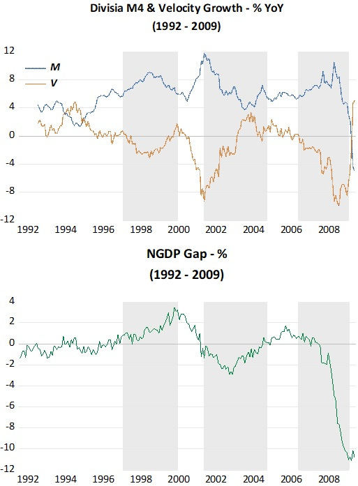
The first chart shows how monetary policy (the workings of the “Thermostst”) performed from 1992 to 2009.

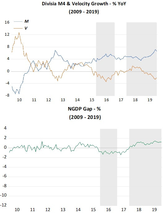
Before the GR, the NGDP gaps tend to be relatively small and dissapear rather quickly because the policy errors are corrected, with money growth more closely offsetting changes in velocity.

Towards the end of the sample, the GR comes about because monetary policy fails completely. When velocity tanks during hightened financial related uncertainties, money growth barely rises. The NGDP gap widens immensely. When the nominal stability is lost, unemployment balloons and real growth dives!

At the very end of the sample, velocity rises quickly and money supply supply growth falls significantly less (even if it becomes negative), so, according to our thermostat analogy, the house temperature that had fallen drastically was allowed to absorb some of heat flowing from the increasing outside temperature.

That was far from enough, however, to take the house temperature back to the previous level, but only enough to keep the house temperature at a permanently cooler level.

In the next chart, covering the period from the end of the GR to just before C-19 hit, we observe that monetary policy did a great job in keeping the house temperature (NGDP) very close to this new “cooler” level, with only minor deviations towards the end of the sample.

Note that during this time unemployment was falling all the way to less than 4%, real growth was stable at around 2% and inflation was also low (below target) and stable. This is completely consistent with what Friedman said; “stabilizing nominal expenditures means stabilizing both inflation and output.”

Given that the NGDP level was lower than the one that prevailed before the GR, and its growth rate also lower (4% vs 5%), the economy was not as strong, with real growth lower than previously (2% vs 3%).

We finally move to the C-19 affected period. The sample is small, but full of “events” (and some records too).

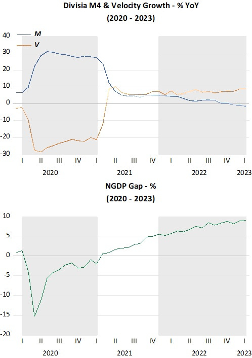
Before becoming a supply shock (lockdowns and supply chain problems), C-19 was a massive monetary shock, this time engendered by a massive increase in money demand (a gargantuan drop in velocity). This time, the thermostat reacted quickly, with the heat (M) rising fast to offset the fall in the outside temperature (V).

That´s the reason the recession that ensued when C-19 hit was the shortest on record and also why the recovery began immediately and a full recovery was in place in the space of just one year after the previous peak.

The first shaded area in the chart below shows this clearly.

It´s interesting to note, and this is clear evidence that looking just at money supply growth does not lead to good analysis, that in Spring 2020 “die-hard” monetarists where shouting very loudely that the record (another one) growth in money supply would be followed by:

Get Ready for the Return of Inflation

Fed actions have increased the quantity of money in the U.S. economy at a blistering rate.

Inflation only went above the 2% target one year later, exactly at the moment an Excess Demand for money (velocity falling faster than the growth in money supply) flipped to an Excess Supply of money (velocity rising faster than the fall in money supply growth). So we don´t see any “lags in effect of monetary policy”.

The monetarist counterargument will surely be “There was 12 or 13 month lag between the “record” increase in money growth and the rise in inflation”. If you stop to think about that argument under the proper view of what monetary policy is, you will conclude that if money supply had not risen at all, or just a little, the economy would have sunk into the deepest recession on record, accompanied by deflation (despite the whatever small increase in money supply)!

The two charts on inflation below show that both Core & Headline PCE inflation have similar shapes.

Headline PCE inflation falls deeper and rises higher than Core PCE because it is “enhanced” by supply shocks! What is notable, again without appealing to “lags in effect”, is that both stop rising and start to fall when the excess supply of money begins to be “worked off” (the RHS shaded areas in the charts).

Now, however, “there´s aproblem, Houston”. The “rocket” climbed above the “ideal trajectory”. What do we do? Should we “force it down”, or should we just “slow its speed and let it travel along the new trajectory”?

These decisions can easily give space to “conspiracy theories” (“CTs”) (sometimes not totally unfounded). For example, after the big monetary mistake that led to the Great Recession, the Fed never allowed the “rocket” to climb to the previous trajectory, just letting it travel along a lower trajectory at a slower speed.

Why? According to “CTs”, if the “rocket” had regained the original trajectory, everyone would have surmised that the “rocket” had dropped due to “pilot” error. Much better the “pilot” be considered a “hero” that avoided a “mortal crash”!

That “CT” is not totally unfounded. For example, Athanasios Orphanides has an interesting story about the 1937 recession within the depression:

Though the extent of the sharp decline in activity was not immediately evident, by Fall it became fully clear to the Committee that the economy was thrown back to a severe recession, once again.

The following evaluation of the situation by (John) Williams at the November 1937 meeting is informative, both for offering a frank admission that the FOMC apparently wished for a slowdown to occur and also for outlining the case that the recession, nonetheless, had nothing to do with the monetary tightening that preceded it.

Particularly enlightening is the reasoning offered by Williams as to why a reversal of the earlier tightening action would be ill advised. We all know how it developed. There was a feeling last spring that things were going pretty fast … we had about six months of incipient boom conditions with rapid rise of prices, price and wage spirals and forward buying and you will recall that last spring there were dangers of a run-away situation which would bring the recovery prematurely to a close. We all felt, as a result of that, that some recession was desirable … We have had continued ease of money all through the depression. We have never had a recovery like that. It follows from that that we can’t count upon a policy of monetary ease as a major corrective. …

In response to an inquiry by Mr. Davis as to how the increase in reserve requirements has been in the picture, Mr. Williams stated that it was not the cause but rather the occasion for the change. … It is a coincidence in time. …

If action is taken now it will be rationalized that, in the event of recovery, the action was what was needed and the System was the cause of the downturn.

It makes a bad record and confused thinking. I am convinced that the thing is primarily non-monetary and I would like to see it through on that ground. There is no good reason now for a major depression and that being the case there is a good chance of a non-monetary program working out and I would rather not muddy the record with action that might be misinterpreted. (FOMC Meeting, November 29, 1937. Transcript of notes taken on the statement by Mr. Williams.)

What a hypocrite! More “CT”: As in 1937, we now also have a John Williams at the (New York)Fed!

So, hopefully, this time around the Fed will also Not allow the “rocket” to go back to the lower trajectory. Hopefully, also, it will not go back to “crising speed” (say 4%-5% YoY NGDP growth (now it is “travelling” at ¨6%-7%) “too fast”. Unfortunately, the Fed has a “hard on” to get back quickly to 2% inflation…! Which reminds ne of James Meade´s argument in his 1977 Nobel Lecture, that “inflation targeting is dangerous”!

Earlier I spoke of ‘price stability’ as being one of the components of ‘internal balance’. Yet in the outline which I have just given of a possible distribution of responsibilities no one is directly responsible for price stability.

To make price stability itself the objective of demand management would be very dangerous. If there were an upward pressure on prices because the prices of imports had risen or because indirect taxes had been raised, the maintenance of price stability would require an offsetting absolute reduction in domestic money wage costs; and who knows what levels of depression and unemployment it might be necessary consciously to engineer in order to achieve such a result?

From this 30-year history, it seems that whenever monetary policy did well it was due to happenstance. Is there a way to do good monetary policy in a way everyone knows “what the hell the Fed is doing”?

A proposal Scott Sumner originally put forth many years ago could satisfy that goal:

Instead, I favor moving toward a regime where we collapse the monetary policy indicator, instrument and goal into one variable—NGDP futures prices. Ideally, NGDP futures prices would be the policy instrument (the thing we target), the policy indicator (the thing we look at to determine the current stance of policy) and the policy goal (with the goal being say 4%/year growth in NGDP futures prices, level targeting.)

Then we can stop doing all these SVAR models.