A 21st Century US Monetary Story

with "money" properly measured

Ten years ago, William Barnett published “Getting it wrong - How faulty monetary statistics undermine the Fed, the Financial System and the Economy”. The book puts together more than 30 years of his research involving the construction of appropriately measured money indicators. The first half of the book is eminently readable, with all the technical details comprising the second half.

What we get are Divisia Monetary Aggregates. The construction of Divisia indices of monetary aggregates takes into account, in establishing changes in the supply of various forms of money, weights according to how liquid each form is and the opportunity cost of holding the different assets. This contrasts with the Simple Sum Monetary Aggregates (like M1, M2, M3, etc.), that have no weighting system, with all forms of money having the same weight (=1).

The book provides dozens of examples that point to the weakness of Simple Sum monetary aggregates. To make my “21st C monetary story easier to follow, I´ll show, with ample illustration, Milton Friedman´s prognosis made on September 26 1983 in his Newsweek column “A case of bad good news”: (page 108 of the book)

President Reagan, politicians of all political persuasions, journalists specializing in economics, Wall Street, the business community—all these and many more are hailing the recent economic statistics showing rapid growth in output and employment as very good news indeed.

One group of economists—the monetarists—are a conspicuous exception. In early 1983, almost to a person economic forecasters were predicting a slow and sluggish recovery. We predicted that “1983 will be a year of rapid and vigorous economic growth.”

That judgment was based on two considerations: the length and severity of the recession that ended in December 1982 [Friedman´s “Plucking Model”], and the monetary explosion that was then in process—a rise in M1 at the annual rate of 15 percent from July 1982 to January 1983.

It seemed to us that “this monetary explosion assures vigorous economic growth in the coming months”—but also that “unfortunately, if it continues much longer, it will also produce a renewed acceleration of inflation and a sharp rise in interest rates.”

The monetary explosion did produce vigorous growth. Unfortunately, it also did continue—at the annual rate of more than 14 percent from January to July. Interest rates have already risen sharply. Inflation has not yet accelerated. That will come next year, since it generally takes about two years for monetary acceleration to work its way through to inflation.

…The monetary explosion from July 1982 to July 1983 leaves no satisfactory way out of our present situation. The Fed’s stepping on the brakes will appear to have no immediate effect. Rapid recovery will continue under the impetus of earlier monetary growth.

With its historical shortsightedness, the Fed will be tempted to step still harder on the brake—just as the failure of rapid monetary growth in late 1982 to generate immediate recovery led it to keep its collective foot on the accelerator much too long. The result is bound to be renewed stagflation—recession accompanied by rising inflation and high interest rates.

Interestingly, on the same date, William Barnett gave an interview to Forbes, which was titled “What explosion”? (page 109 in the book)

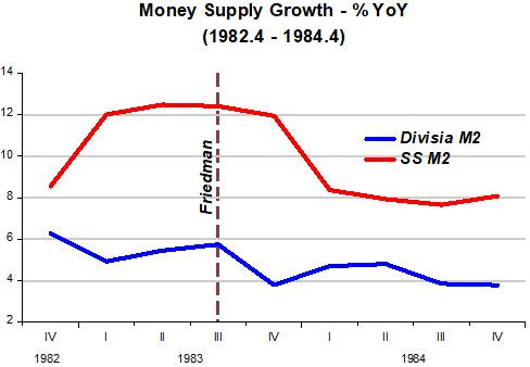
…The other conclusion is that people have been panicking unnecessarily about money supply growth this year. The new bank money funds and the super NOW accounts have been sucking money that was formerly held in other forms…But Divisia aggregates are rising not much different from last year. Thus, the apparent “explosion” can be viewed as a statistical blip.

The chart below shows the drastically different information given out by the two aggregates (Divisia M2 & SS M2).

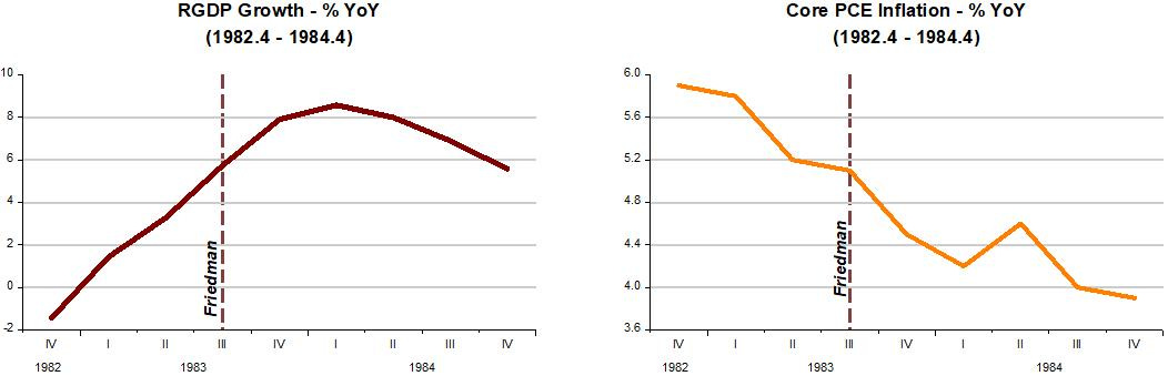
How about Friedman´s predictions for real growth and inflation? Growth remained robust in 1984 (and continued in 1985 and 1986). Inflation fell in 1984 (and continued on a downtrend in 1985 and 1986).

I jump to the 21st Century. The monetary variable is the broadest of the Divisia indices, Divisia M4. The pictures are presented in levels, which I believe make the story clearer, and avoids all the wiggles present when data are presented in growth rate format.

The thread underlying the story is Friedman´s “Thermostat Analogy”, according to which the Fed should operate as a well functioning thermostat, offsetting changes in the “outside temperature” (Velocity) with changes in money supply so as to keep the “inside temperature” (NGDP) stable.

The panel below, covering the past 21 years illustrate.

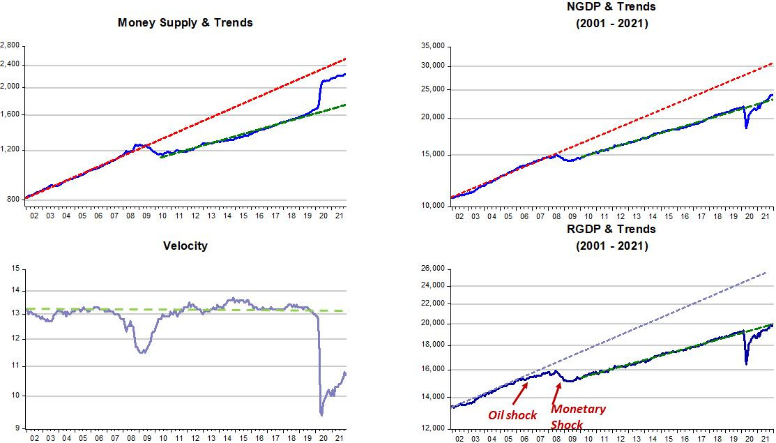
In the first few years of the new century, velocity was stable, money rose at a stable rate and so did aggregate nominal spending (NGDP). RGDP also rose steadily before being impacted by oil shocks.

And then,“something” happened. Maybe the rise in uncertainty revolving around the house and financial sectors, led to a fall in velocity. Instead of offsetting it, the Fed “enhanced” it by letting money supply fall. And when velocity returned to “normal”, the Fed allowed money supply to remain at the lower level.

Not surprisingly, NGDP remained below the previous path, with almost everyone wondering why there was no recovery. At that point, ideas such as “secular stagnation” became popular!

The economy was again stabilized at this lower (“Secular Stagnation”) trend path. The effects of the Fed´s “choice” to travel along a lower trend path were significant. Unemployment took a long time coming down but more importantly, the damage to the labor market in terms of the employment ratio and labor force participation were lasting.

What is notable in the panel above is the contrast between monetary policy in 2008-09 and 2020-21. The first was a “pure” monetary policy shock while the second was a combination of a supply shock (Covid19) and (related to it) a velocity shock.

The first was “Fed made”, while in the second, the Fed reacted fast and forcefully. No surprise, then, that NGDP (and RGDP) quickly travelled back to the original “Secular Stagnation” trend. Unemployment dropped vertiginously, resembling those divers from the rock faces in Acapulco.

A zoom on the more recent period is illustrative.

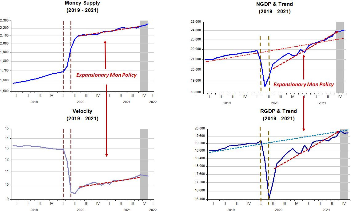
The drop in velocity was sudden and deep. The Fed reacted quickly. The recession was the shortest on record (2 months!). Following the recession trough in April 2020, monetary policy became expansionary. Both money supply and velocity were rising.

With the money supply growth that reached 30% YoY in June, the conventional monetarists went ballistic as early as Spring 2020, predicting a strong rise in inflation in 2021/22.

What they completely ignored was the huge drop in velocity. Just imagine if money supply growth had not increased. Instead of facing some increase in inflation we would be facing the biggest depression in history!

My take is that inflation was a "problem" that substituted for a second Great Depression, that would likely have materialized if "old monetarists" had had their way! And it mostly came about because of the overhanging supply restrictions.

The next figures take a look at the interplay of inflation, supply constraints and monetary policy (the stance of which is defined by the behavior of NGDP). We look at three categories of PCE inflation. The headline which, in addition to energy and food prices is impacted by “Covid19-related” prices, the core PCE, which “avoids” energy & food, but is also impacted by “Covid19-related” prices and the trimmed PCE, which mostly reflects “Covid19-free” prices.

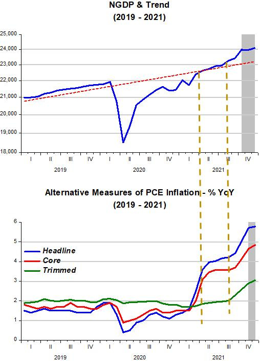
Note that when the expansionary monetary policy brought NGDP back close to trend, supply constraints became binding and those measures of inflation “Covid19-related”, went up. The “Covid19-free” inflation measure remained flat.

Importantly, as illustrated between the two dashed lines, when NGDP increases according to trend, all inflation measures flatten out, only increasing when monetary policy becomes expansionary again. At that point, even the “Covid19-free” prices increase, leading me to conclude that is the point where monetary policy becomes “unwantedly expansionary”.

More recently (shaded area), NGDP stops rising and inflation indicators show a kink, beginning to flatten. This may have been “luck”. Velocity ticked down and money supply just offset it, flattening NGDP.

My (conservative) assumption is that the Fed will “work” to keep NGDP flat until it reaches the “Great Stagnation” trend. Inflation will remain elevated for some months, before dropping when supply constraints wane. The trimmed PCE, which has only reached 3% YoY, will likely fall faster due to monetary policy becoming “neutral”.

My bottom-line, to repeat is: Don´t forget that the “uncomfortable” inflation being experienced was the price paid to avoid a “deadly” depression!

Note: Divisia Monetary Indices can be found here, while monthly GDP numbers can be found here.

If you´ve come this far and found it useful or enjoyable, please subscribe. And why not share with friends and acquaintances!